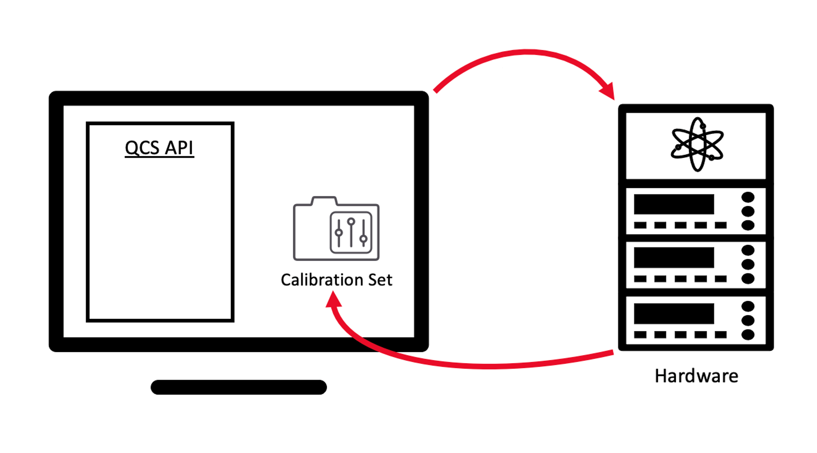
Experiments#
This section walks you through creating experiments from scratch and executing a basic
calibration workflow for a two-level quantum system using QCS’s built-in experiment
routines. These routines are built around the Experiment
and CalibrationExperiment classes, which are designed
to help users execute programs on Keysight hardware and streamline the analysis of results.
Users can either take advantage of the pre-designed experiments available in QCS or create
their own custom experiments using these classes by following the steps in this guide.
The purpose of the Experiment class is to facilitate the development of common user
experiments and calibration routines. The latter in particular can be achieved through
a subclass called CalibrationExperiment. Now, let’s examine how
to use each of these classes and identify the most suitable scenarios for each.
Note
For a comprehensive demonstration, including a downloadable Jupyter notebook showing visualizations and analysis methods on experimental data refer to one of the guides on built-in experiments in this section (see Available built-in experiments).
Experiment#
This guide outlines the steps for defining, executing, and plotting data from a QCS experiment on hardware.
Instantiating a new Experiment#
Setting up#
We start by initializing a qubit. Experiments require the use of a ChannelMapper
to indicate how qudits are addressed via hardware channels. For a basic setup, see
Channel Mapper, here we define an empty one for demonstration.
We then use a make_calibration_set() function that
generates a CalibrationSet for a given number of qubits.
“<ip_address>” can be omitted if the code is run locally on the PC that serves as the controller for the QCS. Otherwise, adding the IP address of the controller PC allows users to remotely submit jobs from any computer connected to the network.
import keysight.qcs as qcs
import numpy as np
from keysight.qcs.experiments import Experiment, make_calibration_set


n_qubits = 1
qubits = qcs.Qudits(range(n_qubits))
mapper = qcs.ChannelMapper("<ip_address>")
calibration_set = make_calibration_set(n_qubits)
Defining a program#
Let’s create a simple program with operations to run while executing the experiment.
Here the program is a pulse on the xy_channels followed
by a measurement.
program = qcs.Program()
amplitude = qcs.Scalar("amplitude", dtype=float)
waveform = qcs.RFWaveform(duration = 20e-9, envelope = qcs.GaussianEnvelope(), amplitude = np.pi*amplitude, rf_frequency = 5.1e9)
n_channels = 1
channels = qcs.Channels(range(n_channels), "xy_channels", absolute_phase=False)
program.add_waveform(waveform, channels)
program.add_measurement(qubits)
To ensure that the program behaves as intended, the draw() method can be used.
This method generates an HTML representation of the program.
program.draw()
Adding Fitter and Preprocessor#
For subsequent analysis of experimental data, the Experiment
class allows you to specify a fitter and a preprocessor as parameters.
Fitting involves selecting an appropriate model to extract key parameters from the data, while preprocessing
is used to clean and organize the raw data prior to fitting, ensuring more accurate and robust results.
Users can choose from one of the built-in fitters:
or create a custom one using BaseFitter.
In the same way, the user can choose from one of the built-in Preprocessor:
or create a custom one.
Here we choose two of the built-in ones for demonstration purposes:
from keysight.qcs.analysis import DecayingSinusoid, IQuadrature

fitter = DecayingSinusoid()
pre_processor = IQuadrature()
Declaring the Experiment#
We create an instance of the Experiment class using the
program and the analysis methods we just defined. Note that an experiment can
be executed on a subset of qubits of the calibration set, specified by the targets property.
experiment = Experiment(
                backend = mapper,
                calibration_set = calibration_set,
                targets = qubits,
                program = program,
                fitter = fitter,
                pre_processor = pre_processor,
                name = "Demo Experiment"
                )
The last step of creating an experiment is to configure the repetitions which is done using
configure_repetitions(). This method accepts the
number of shots, a boolean to determine whether the sweep should be performed in hardware or software time,
and the values over which to sweep.
experiment.configure_repetitions(
                n_shots=100,
                hw_sweep=True,
                amplitude=np.linspace(0, 1.0/np.pi, 100)
                )
to configure “nested” sweeps on your experiment the synthax is as follow:
experiment.configure_repetitions(
                n_shots=100,
                hw_sweep=True,
                readout_frequencies= frequency_scan,
                readout_pulse_amplitudes= amplitude_scan,
                )
Lastly to configure “zipped” or “simultaneous” sweeps on your experiment the synthax is:
experiment.configure_repetitions(
                n_shots=100,
                hw_sweep=True,
                variables = ["x180_pulse_amplitudes", "xy_pulse_frequencies"],
                values = [amp_scan_values, freq_scan_values]
                )
Executing and retrieving results#
To execute this experiment, we can simply run execute().
We can provide the name of the experiment during execution:
experiment.execute(name="Demo Experiment with 100 shots")
To obtain a Dataframe of the experimental data associated to this executed experiment,
we can use the get_trace_pandas(), get_classified_pandas() or the get_iq_pandas() method
like a standard QCS program:
dataframe = experiment.get_iq_pandas()
Visualization#
There are several ways of visualizing the data.
Like QCS programs, experiments also have the plot_trace(), the plot_spectrum()
and the plot_iq() methods.
experiment.plot_iq()
Additionally, the experiment also has the
plot() method that plots both the
experiment data and the fit (if a fitter was specified). This method also contains an
interactive widget that lets the user modify the initial guess used for the fit when
setting interactive_plot=True.
To visualize the fit of an experiment with a two-dimensional sweep, the user must
specify which sweep parameter to use as the outer loop via the second_sweep_name
argument. The remaining parameter will define the x-axis for fitting. If no fitter or
preprocessor is provided, the raw I/Q data is plotted by default. If I/Q data is
unavailable, trace data is shown instead.
To improve the visual smoothness of the fitted model plot, especially when x_values are
sparse or widely spaced, the plot_density parameter can be used to densify the
x-axis. It inserts interpolated points between each pair of existing x_values, resulting
in a smoother curve. This integer parameter affects only the display of the fitted
model—not the fitting itself. By default, plot_density is set to 0 and capped
at 50.
experiment.plot()
Calibration Experiment#
A CalibrationExperiment is a subclass of Experiment
and is used to facilitate the calibration of variables on the calibration set.
Here we outline the entire process of defining a calibration experiment, from the initial setup to plotting the data obtained from the experiment.
Instantiating a new Calibration Experiment#
Setting up#
First, we initialize a qubit and a ChannelMapper.
Then, we create a CalibrationSet using the
make_calibration_set() function, as demonstrated in the Experiment section.
import keysight.qcs as qcs
import numpy as np
from keysight.qcs.experiments import CalibrationExperiment, make_calibration_set
from keysight.qcs.quantum import PAULIS


n_qubits = 1
qubits = qcs.Qudits(range(n_qubits))
mapper = qcs.ChannelMapper("<ip_address>")
calibration_set = make_calibration_set(n_qubits)
Defining a program#
Let’s create a simple program with operations to run while executing the experiment.
Here the program is a pulse on the xy_channels followed
by a measurement.
program = qcs.Program()
amplitude = qcs.Array("x180_pulse_amplitudes", shape=(len(qubits),), dtype=float)
program.add_parametric_gate(PAULIS.rx, [np.pi * amplitude], qubits)
program.add_measurement(qubits)
To ensure that the program behaves as intended, the draw() method can be used.
This method generates an HTML representation of the program.
program.draw()
Choosing the operation to calibrate#
The CalibrationExperiment includes an additional parameter
called operation, which specifies the operation to be calibrated in the experiment.
The name of this operation need to match the name of the linker defined in the calibration set.
In this example, we are calibrating the operation “x”, which corresponds to the X gate
linker. This can be defined in the calibration set as follows:
x_pulse = RFWaveform(
    xy_pulse_durations,
    GaussianEnvelope(),
    x180_pulse_amplitudes,
    xy_pulse_frequencies,
)
calibration_set.add_sq_gate("x", GATES.x, x_pulse, qubits, xy_pulse_channels)
Note
For more information on linkers, refer to Linkers
Declaring the Calibration Experiment#
We create an instance of the CalibrationExperiment class using the
program we just defined (and the same fitter and preprocessor we used for Experiment).
calibration_experiment = CalibrationExperiment(
                            backend = mapper,
                            calibration_set = calibration_set,
                            operation = "x",
                            qudits = qubits,
                            program = program,
                            fitter = fitter,
                            pre_processor = pre_processor
                            )
Note
The targets should be a subset of the linker’s targets.
The last step of creating an experiment is to configure the repetitions which is done using
configure_repetitions(). This method accepts the
number of shots, a boolean to determine whether the sweep should be performed in hardware or software time,
and the values over which to sweep. In addition to sweeping variables on the experiment program,
configure_repetitions can be used to sweep variables contained on the corresponding linker’s program.
Note
To sweep the correct variable, specify its name in the arguments of configure_repetitions
using the format **{<variable_name>: <variable_values>}.
variable_name = "x180_pulse_amplitudes"
variable_scan = np.linspace(0, 1.0/np.pi, 100)
calibration_experiment.configure_repetitions(
                            n_shots=100,
                            hw_sweep=True,
                            **{variable_name: variable_scan}
                            )
Executing, retrieving results and visualization#
The methods presented for the Experiment can be used the same exact way
for a CalibrationExperiment.
Handling calibration values#
CalibrationExperiment includes two additional methods that
simplify the process of updating calibration parameters:
These are get_updated_calibration_values()
and set_updated_calibration_values().
get_updated_calibration_values()generates a dictionary mapping variable names (strings) to numbers or arrays.set_updated_calibration_values()updates the calibration_set that is on the experiment, either with input values or the return fromget_updated_calibration_values().
Note
When designing a custom CalibrationExperiment, you need to define
get_updated_calibration_values() since there is
no general method and it varies between experiments. You can find examples of its implementation in Available built-in experiments
The typical workflow for using these methods is then:
calibration_experiment.get_updated_calibration_values()
This will return a dictionary where the calibrated variable_name is the key, and the
corresponding values for the target qubits are the values, such as {'variable_name': 0.4967}.
The user can check the current state of the variable in the calibration set prior to its update as follows:
calibration_experiment.calibration_set.variables.<variable_name>.value
This will return an array containing the previous value(s) of that variable (for example array([0.5])). We can then proceed to
update it as follows:
calibration_experiment.set_updated_calibration_values()
calibration_experiment.calibration_set.variables.<variable_name>.value
This will now output array([0.4967]), thus confirming that the variable has been updated.
Note
The updated calibration set can be saved using export_values()
method as shown in Managing calibration data and linkers
Available built-in experiments#
Note
The following examples utilize the assets
calibration set and
channel mapper which can be generated
with the scripts calibration.py and
channel_mapper.py.
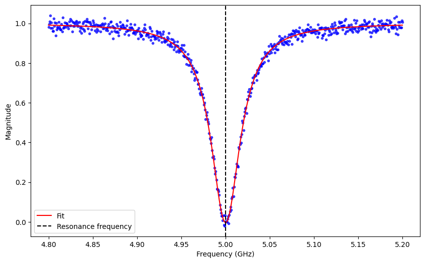
Resonator Spectroscopy
Resonator Spectroscopy experiments allow users to calibrate the parameters of the readout pulse for the measurement operation.
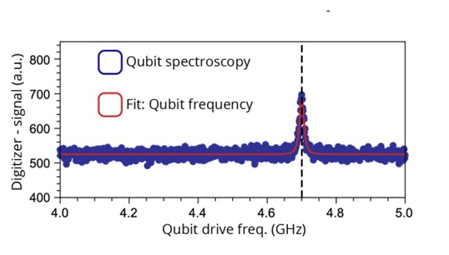
Qubit Spectroscopy
Qubit Spectroscopy experiments allow users to calibrate the driving frequency of qubit control pulses.
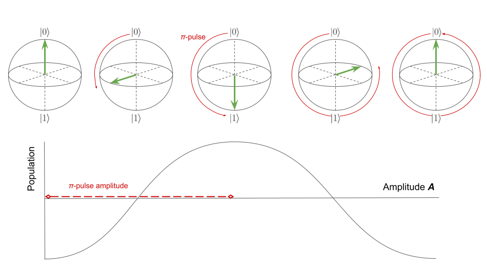
Rabi
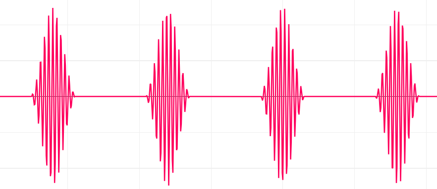
Rabi experiments allow users to calibrate the amplitude of \(\pi\)-pulses.
Error Amplification
Error Amplification experiments allow users to fine-tune the amplitude of \(\pi\)-pulse determined during the Rabi experiment to achieve better accuracy.
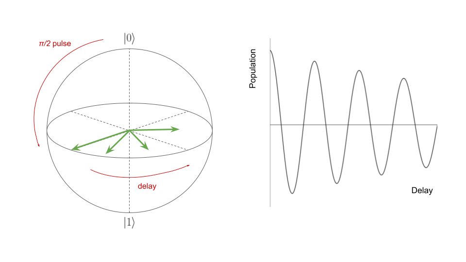
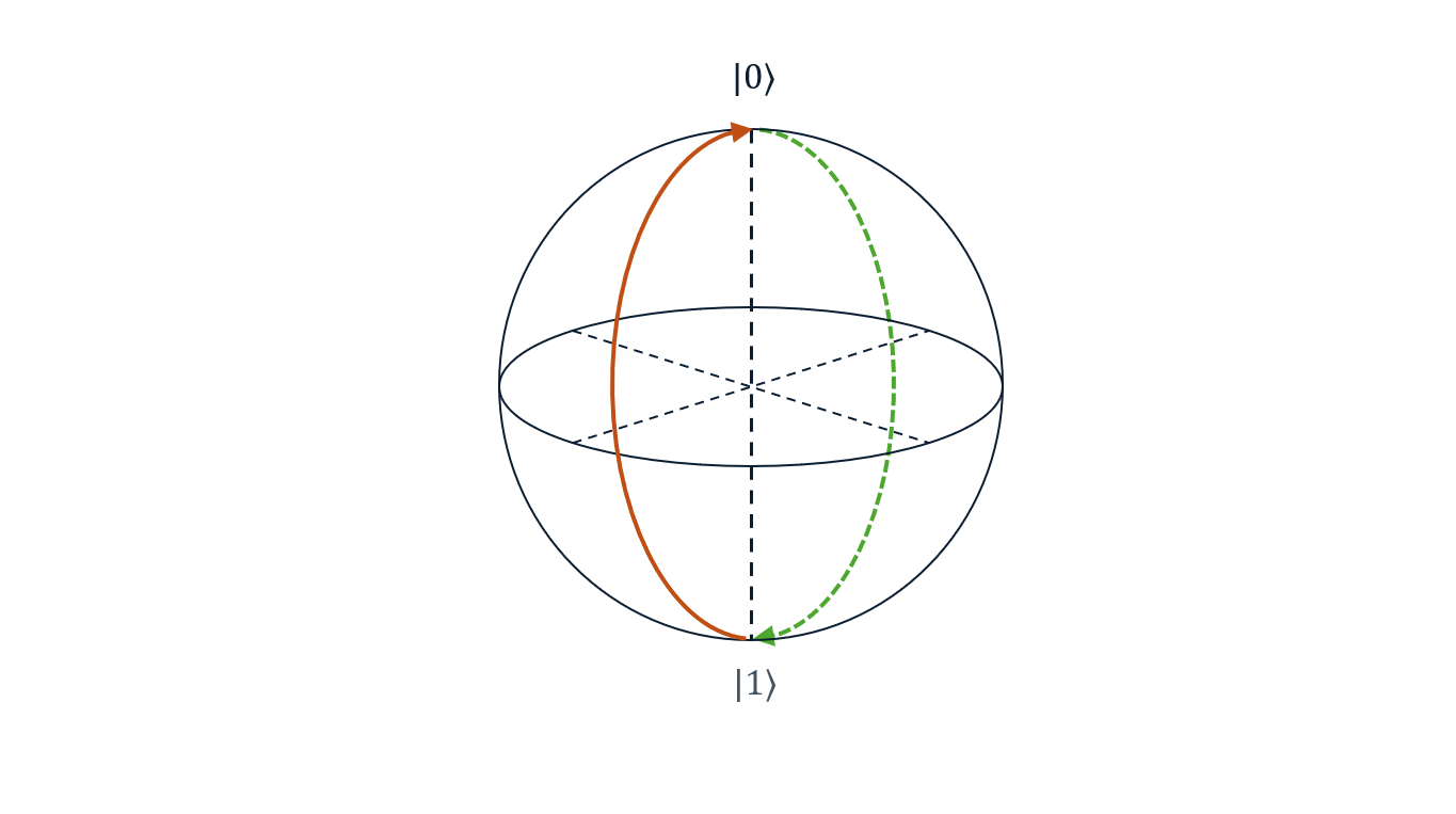
Coherence
Coherence experiments allow users to learn a characteristic noise time scale for a qubit.
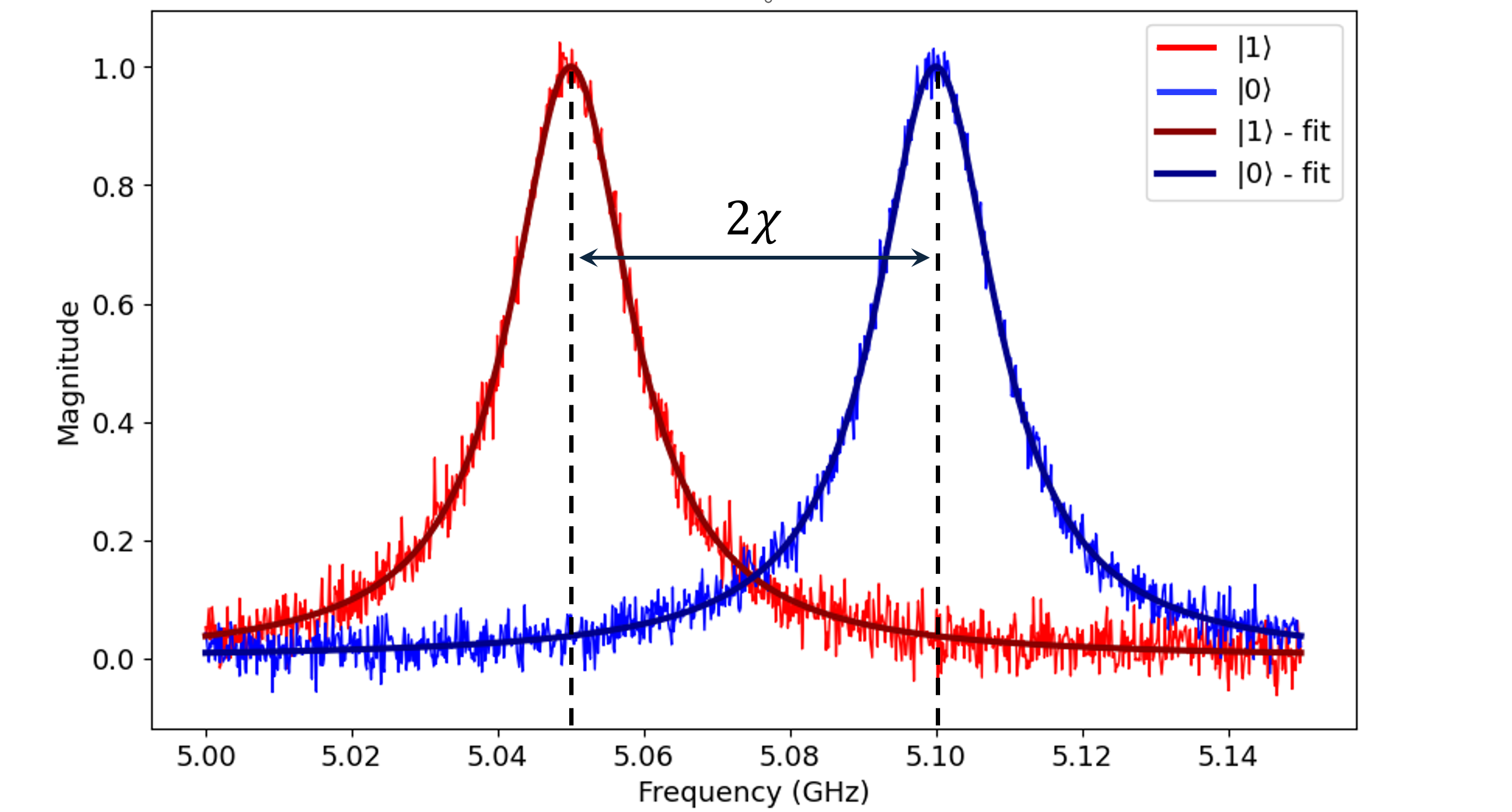
Dispersive Shift
Dispersive Shift experiments allow users to learn how the qubit’s state influences the resonance frequency of the readout resonator.
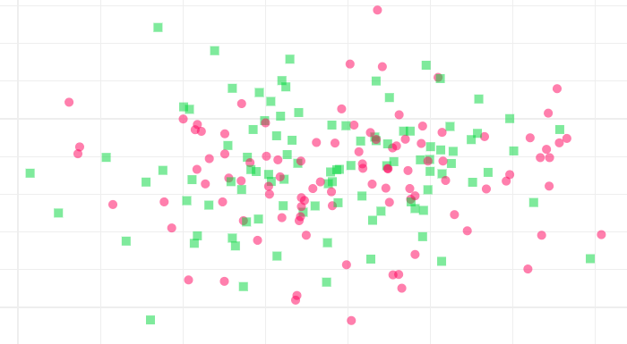
IQ Distribution
IQ Distribution experiments allow users to measure the I/Q distribution of both the ground state and excited state.
Dynamical Decoupling
Dynamical Decoupling experiments allow users to improve decoherence times by sending a series of pulses with certain intervals are applied to the qubits, effectively decouple them from their environment.
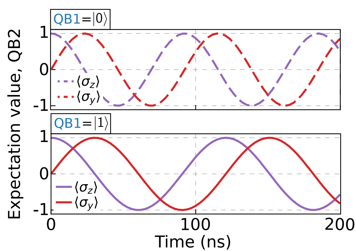
Cross Resonance
Cross Resonance experiment is a two-qubit experiment that allows users to calibrate the amplitude of the Cross Resonance pulse sent on the control qubit.
Philip Krantz, Morten Kjaergaard, Fei Yan, Terry Orlando, Simon Gustavsson, and William Oliver. A quantum engineer's guide to superconducting qubits. 2019. arXiv:1904.06560.