---

Download

Download this file as Jupyter notebook: qubit_coherence.ipynb.

Coherence characterization

Note

The assets are set up to map a maximum of 4 qudits to a single physical AWG and digitizer channel with an LO frequency of 5.5 GHz. For the purposes of this demonstration, we connect the output of the AWG to the digitizer so we can capture both the control and readout pulses.

Coherence characterization experiments uses varying delays to probe the dynamic properties of the qubit. Here we give a guide to show how to perform a Ramsey Experiment, a Hahn Echo Experiment and a Relaxation experiment.

import keysight.qcs as qcs
import numpy as np
from keysight.qcs.experiments import RamseyExperiment, EchoExperiment, T1Experiment
from keysight.qcs.experiments import make_calibration_set

Relaxation Experiment

Another example of decoherence is thermal relaxation which happens at a time scale commonly referred to as T1. This section shows how to perform a Relaxation experiment to learn that decay time T1 using the class T1Experiment.

A \(\pi\) gate is first applied to a qubit in the ground state to bring it to the excited state followed by a varying delay. The sequence is then followed by a readout pulse.

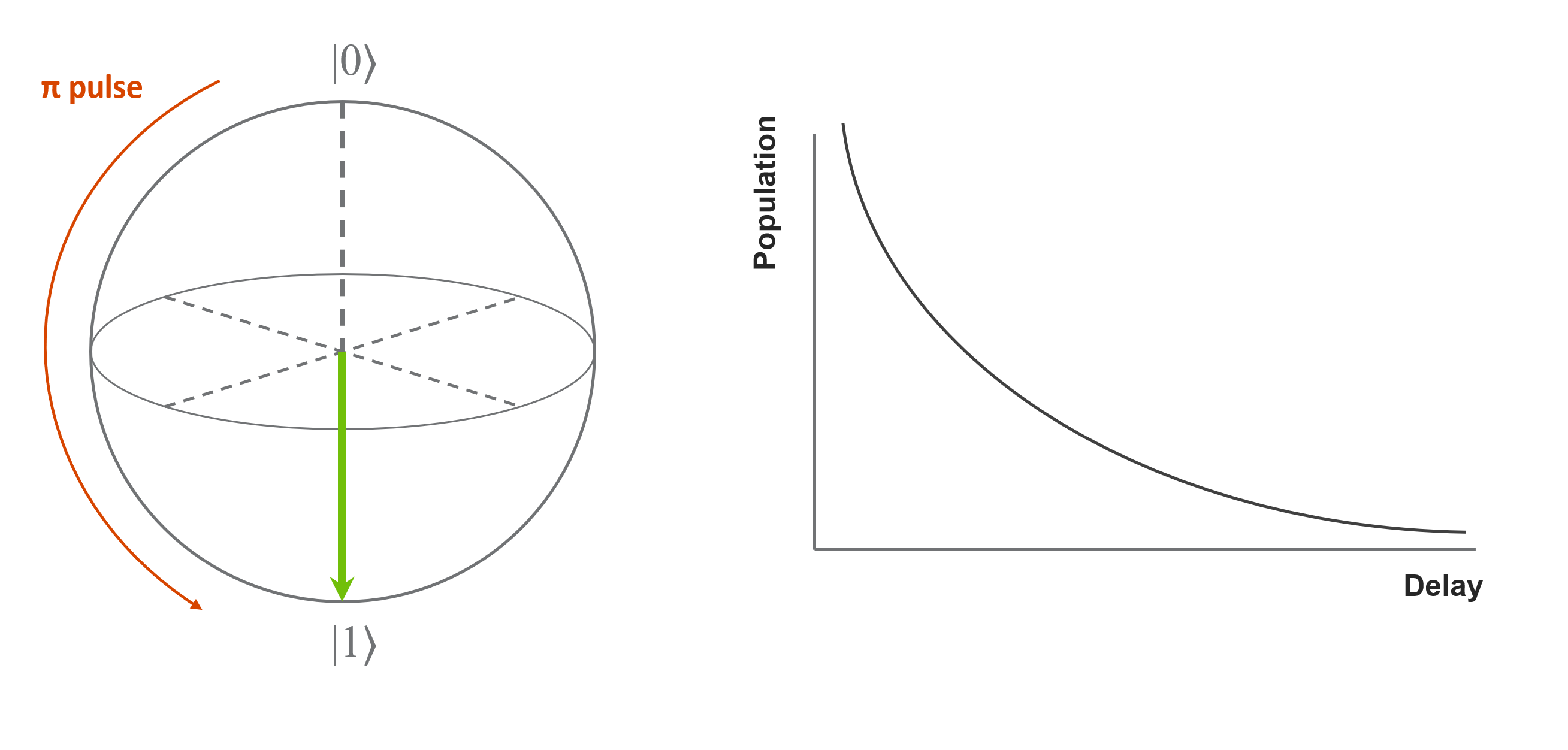
This experiment follows the following steps:

1. Initialize the qubit to the excited state by applying a \(\pi`\)

2. Apply a delay.

3. Measure the population of the qubit in the excited state.

4. Repeat the above steps with varying delay time.

We start again by initializing a qubit and loading a channel mapper to create a new instance of the T1Experiment class. Next, we generate a calibration set for the qubit using make_calibration_set(). This file includes the quantum operations and variables we will need to run the experiment.

# set the following to True when connected to hardware
run_on_hw = False

n_qubits = 1
qubits = qcs.Qudits(range(n_qubits))
calibration_set = make_calibration_set(n_qubits)

# generate an empty channel mapper
mapper = qcs.ChannelMapper("ip_addr")

# create a T1 experiment
t1_experiment = T1Experiment(mapper, calibration_set=calibration_set, qubits=qubits)

t1_experiment.draw()

# The program consists of one `X` gate with a variable delay followed by a measurement.
#

		Program Program Duration undefined Layers 1 Targets 1 Repetitions
		Layer #0 Layer #0 Duration undefined
qudits	0	X Gate X on ('qudits', 0) Matrix: 0 1 1 0	Delay on ('qudits', 0) Parameters Duration Array(name=pulse_delay, shape=(1,), dtype=float, unit=s)	Measure on ('qudits', 0) Parameters Dim 2

# configure the repetitions for this experiment
start_delay = 40e-9
end_delay = 80e-9
steps = 3
scan_values = np.linspace([start_delay] * n_qubits, [end_delay] * n_qubits, steps)
t1_experiment.configure_repetitions(delays=scan_values, n_shots=1)

Note

We can set different delay values for different qubits, as long as every qubit gets the same number of values i.e. delays should have shape (steps, n_qubits).

Compiling this program to the waveform level using the ParameterizedLinkers in the calibration set results in the following program:

t1_experiment.compiled_program.draw()

		Program Program Duration undefined Layers 1 Targets 3 Repetitions Repeat with 1 repetitions Sweep with 3 repetitions Associations pulse_delay Array(name=_implicit, shape=(3, 1), dtype=float, unit=none, value=[[40 ns], [60 ns], [80 ns]])
		Layer #0 Layer #0 Duration undefined
xy_pulse	0	RFWaveform on ('xy_pulse', 0) Parameters Duration ScalarRef(name=xy_pulse_durations, value=30 ns, dtype=float, unit=s) Amplitude ScalarRef(name=x180_pulse_amplitudes, value=0.5, dtype=float, unit=none) Frequency ScalarRef(name=xy_pulse_frequencies, value=5.1 GHz, dtype=float, unit=Hz) Envelope GaussianEnvelope(2.0) Instantaneous Phase ScalarRef(name=x_phase, value=0 rad, dtype=float, unit=rad) Post-phase ScalarRef(name=x_post_phase, value=0 rad, dtype=float, unit=rad)	Delay on ('xy_pulse', 0) Parameters Duration Max(ScalarRef(name=readout_pulse_duration, value=100 ns, dtype=float, unit=s), ScalarRef(name=acquisition_duration, value=100 ns, dtype=float, unit=s))
readout_pulse	0	Delay on ('readout_pulse', 0) Parameters Duration Array(name=_implicit, shape=(1,), dtype=float, unit=s)	RFWaveform on ('readout_pulse', 0) Parameters Duration ScalarRef(name=readout_pulse_duration, value=100 ns, dtype=float, unit=s) Amplitude ScalarRef(name=readout_pulse_amplitudes, value=0.1, dtype=float, unit=none) Frequency ScalarRef(name=readout_frequencies, value=5.15 GHz, dtype=float, unit=Hz) Envelope SineEnvelope() Instantaneous Phase ScalarRef(name=measurement_phase, value=0 rad, dtype=float, unit=rad) Post-phase ScalarRef(name=measurement_post_phase, value=0 rad, dtype=float, unit=rad)	Delay on ('readout_pulse', 0) Parameters Duration Scalar(name=_implicit, value=0 s, dtype=float, unit=s)
readout_acquisition	0	Delay on ('readout_acquisition', 0) Parameters Duration Array(name=_implicit, shape=(1,), dtype=float, unit=s)	Acquisition on ('readout_acquisition', 0) Parameters Duration ScalarRef(name=acquisition_duration, value=100 ns, dtype=float, unit=s) Integration Filter RFWaveform Parameters Duration ScalarRef(name=acquisition_duration, value=100 ns, dtype=float, unit=s) Amplitude ScalarRef(name=measurement_integrator_amplitude, value=1, dtype=float, unit=none) Frequency ScalarRef(name=readout_frequencies, value=5.15 GHz, dtype=float, unit=Hz) Envelope ConstantEnvelope() Instantaneous Phase ScalarRef(name=measurement_integrator_phase, value=0 rad, dtype=float, unit=rad) Post-phase ScalarRef(name=measurement_integrator_post_phase, value=0 rad, dtype=float, unit=rad) Classifier Classifier(Array(name=references, shape=(1, 2), dtype=complex, unit=none))	Delay on ('readout_acquisition', 0) Parameters Duration Scalar(name=_implicit, value=0 s, dtype=float, unit=s)

We again use the render method to visualize this with the ChannelMapper.

t1_experiment.compiled_program.render(
    channel_subplots=False,
    lo_frequency=5e9,
    sweep_index=2,
    sample_rate=5e9,
)

The sweep index allows you to visualize the change of delay value between the control and readout pulses.

t1_experiment.compiled_program.render(
    channel_subplots=False,
    lo_frequency=5e9,
    sweep_index=0,
    sample_rate=5e9,
)

To execute this experiment, we can simply run

if run_on_hw:
    t1_experiment.execute()
else:
    # load in a previously executed version of this experiment
    t1_experiment = qcs.load("T1Experiment.qcs")

For the purposes of this demonstration, we added a second “ancilla” qubit to the program and connected the physical output channels for our qubit to the digizer associated with the ancilla to allow us to capture the full pulse sequence.

t1_experiment.draw()

		Program Program Duration undefined Layers 1 Targets 2 Repetitions Sweep with 3 repetitions Associations pulse_delay Array(name=_implicit, shape=(3,), dtype=float, unit=none, value=[40 ns, 60 ns, 80 ns]) Repeat with 1 repetitions
		Layer #0 Layer #0 Duration undefined
qudits	0	X Gate X on ('qudits', 0) Matrix: 0 1 1 0	Delay on ('qudits', 0) Parameters Duration Scalar(name=pulse_delay, value=None, dtype=float, unit=s)	Measure on ('qudits', 0) Parameters Dim 2
ancilla	1	Measure on ('ancilla', 1) Parameters Dim 2

We can see the program compiled to the waveform level with the following command:

t1_experiment.compiled_program.draw()

		Program Program Duration undefined Layers 1 Targets 4 Repetitions Sweep with 3 repetitions Associations pulse_delay Array(name=_implicit, shape=(3,), dtype=float, unit=none, value=[40 ns, 60 ns, 80 ns]) Repeat with 1 repetitions
		Layer #0 Layer #0 Duration undefined
xy_pulse	0	RFWaveform on ('xy_pulse', 0) Parameters Duration ScalarRef(name=xy_pulse_durations, value=30 ns, dtype=float, unit=s) Amplitude ScalarRef(name=x180_pulse_amplitudes, value=0.5, dtype=float, unit=none) Frequency ScalarRef(name=xy_pulse_frequencies, value=5.1 GHz, dtype=float, unit=Hz) Envelope GaussianEnvelope(2.0) Instantaneous Phase ScalarRef(name=x_phase, value=0 rad, dtype=float, unit=rad) Post-phase ScalarRef(name=x_post_phase, value=0 rad, dtype=float, unit=rad)	Delay on ('xy_pulse', 0) Parameters Duration Max(ScalarRef(name=readout_pulse_duration, value=220 ns, dtype=float, unit=s), ScalarRef(name=acquisition_duration, value=220 ns, dtype=float, unit=s))
readout_pulse	0	Delay on ('readout_pulse', 0) Parameters Duration Scalar(name=_implicit, value=None, dtype=float, unit=s)	RFWaveform on ('readout_pulse', 0) Parameters Duration ScalarRef(name=readout_pulse_duration, value=100 ns, dtype=float, unit=s) Amplitude ScalarRef(name=readout_pulse_amplitudes, value=0.1, dtype=float, unit=none) Frequency ScalarRef(name=readout_frequencies, value=5.15 GHz, dtype=float, unit=Hz) Envelope SineEnvelope() Instantaneous Phase ScalarRef(name=measurement_phase, value=0 rad, dtype=float, unit=rad) Post-phase ScalarRef(name=measurement_post_phase, value=0 rad, dtype=float, unit=rad)	Delay on ('readout_pulse', 0) Parameters Duration Scalar(name=_implicit, value=120 ns, dtype=float, unit=s)
readout_acquisition	0	Delay on ('readout_acquisition', 0) Parameters Duration Scalar(name=_implicit, value=None, dtype=float, unit=s)	Acquisition on ('readout_acquisition', 0) Parameters Duration ScalarRef(name=acquisition_duration, value=220 ns, dtype=float, unit=s) Integration Filter RFWaveform Parameters Duration ScalarRef(name=acquisition_duration, value=220 ns, dtype=float, unit=s) Amplitude ScalarRef(name=measurement_integrator_amplitude, value=1, dtype=float, unit=none) Frequency ScalarRef(name=readout_frequencies, value=5.15 GHz, dtype=float, unit=Hz) Envelope ConstantEnvelope() Instantaneous Phase ScalarRef(name=measurement_integrator_phase, value=0 rad, dtype=float, unit=rad) Post-phase ScalarRef(name=measurement_integrator_post_phase, value=0 rad, dtype=float, unit=rad) Classifier Classifier(Array(name=references, shape=(1, 2), dtype=complex, unit=none))	Delay on ('readout_acquisition', 0) Parameters Duration Scalar(name=_implicit, value=0 s, dtype=float, unit=s)
	1	Acquisition on ('readout_acquisition', 1) Parameters Duration Scalar(name=_implicit, value=220 ns, dtype=float, unit=s) Integration Filter DCWaveform Parameters Duration Scalar(name=_implicit, value=220 ns, dtype=float, unit=s) Amplitude 1 Frequency 0 Hz Envelope ConstantEnvelope() Instantaneous Phase 0 Post-phase 0

Here we can see the control pulse and the readout pulse separated by our varying delay.

t1_experiment.render(channel_subplots=False, sweep_index=2)

The ancilla qubit is mapped to the digitizer channel 1 and has a single acquisition that spans the duration of both control pulses and the maximum delay between them.

t1_experiment.plot_trace(channels=qcs.Qudits(1, "ancilla"))

Ramsey Experiment

This section shows how to perform a Ramsey experiment to learn the dephasing time of a qubit. This experiment can be easily generated with RamseyExperiment.

Following the Qubit spectroscopy and Rabi experiment, we have determined the qubit’s resonance frequency and \(\pi\)-pulse amplitude which were stored in the calibration set. Given these, we are now able to implement the \(\frac{\pi}{2}\) gate to create an equal superposition between the ground and excited state.

In this guide, we begin characterizing the intrinsic noise of the system by learning the decay rate of the coherence between the ground and excited states of the qubit. The time scale associated with this decoherence is commonly referred to as the \(T_2^*\) time. The Ramsey experiment can also be used to measure the error in the measured resonance frequency of the qubit (the detuning frequency), and further tune up the calibration parameters.

A \(\frac{\pi}{2}\) gate applied to a qubit in the ground state creates an equal superposition state, shown below as a point on the \(XY\) plane of the Bloch sphere. The phase of the state evolves in time, corresponding to a natural precession around the \(Z\) axis. At the same time, dephasing occurs as the state shrinks on the Bloch sphere towards the center (the completely mixed state). After some time has elapsed, a second \(\frac{\pi}{2}\) gate can be applied to drive the qubit to either the ground or excited state. The magnitude of the dephasing can then be measured as the population in the excited state. The rotation shows up in the measurement as an oscillation between the ground and excited states, while the dephasing appears as an exponentially decaying envelope. By varying the delay time, we can learn the characteristic time scale of the decay.

If the offset perfectly corrects the intrinsic rotation, we would not observe any oscillation. In practice, the observed oscillation can be used to recalibrate the qubit’s resonance frequency.

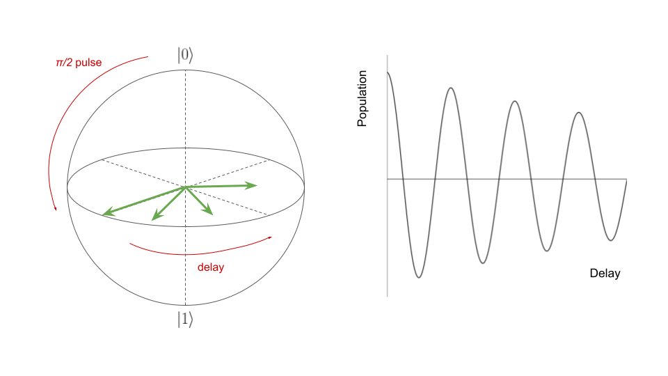
To learn the \(T_2^*\) time and detuning frequency, we perform a Ramsey experiment as follows:

1. Initialize the qubit to an equal superposition state between the ground and excited state (in the \(XY\) plane of the Bloch sphere) by applying a \(\frac{\pi}{2}\) gate.

2. Apply a delay.

3. Apply a second \(\frac{\pi}{2}\) gate to drive the qubit toward either the ground or excited state.

4. Measure the population of the qubit in the excited state.

5. Repeat the above steps with varying delay time.

We start by initializing a qubit and loading a channel mapper to create a new instance of the RamseyExperiment class. Next, we generate a calibration set for the qubit using make_calibration_set(). This file includes the quantum operations and variables we will need to run the experiment.

# set the following to True when connected to hardware
run_on_hw = False

n_qubits = 1
qubits = qcs.Qudits(range(n_qubits))
calibration_set = make_calibration_set(n_qubits)

# generate an empty channel mapper
mapper = qcs.ChannelMapper("ip_addr")

# create Ramsey experiment
ramsey_experiment = RamseyExperiment(
    mapper, calibration_set=calibration_set, qubits=qubits
)

ramsey_experiment.draw()

# The program consists of two simple `X90` gates separated by a variable delay
#  followed by a measurement.

		Program Program Duration undefined Layers 2 Targets 1 Repetitions
		Layer #0 Layer #0 Duration undefined			Layer #1 Layer #1 Duration undefined
qudits	0	X90 Gate X90 on ('qudits', 0) Matrix: 0.71 -0.71j -0.71j 0.71	Delay on ('qudits', 0) Parameters Duration Array(name=pulse_delay, shape=(1,), dtype=float, unit=s)	X90 Gate X90 on ('qudits', 0) Matrix: 0.71 -0.71j -0.71j 0.71	Measure on ('qudits', 0) Parameters Dim 2

# configure the repetitions for this experiment
start_delay = 40e-9
end_delay = 80e-9
steps = 3
scan_values = np.linspace([start_delay] * n_qubits, [end_delay] * n_qubits, steps)
ramsey_experiment.configure_repetitions(delays=scan_values, n_shots=1)

Compiling this program to the waveform level using the ParameterizedLinkers in the calibration set results in the following program:

ramsey_experiment.compiled_program.draw()

		Program Program Duration undefined Layers 2 Targets 3 Repetitions Repeat with 1 repetitions Sweep with 3 repetitions Associations pulse_delay Array(name=_implicit, shape=(3, 1), dtype=float, unit=none, value=[[40 ns], [60 ns], [80 ns]])
		Layer #0 Layer #0 Duration undefined			Layer #1 Layer #1 Duration 100 ns
xy_pulse	0	RFWaveform on ('xy_pulse', 0) Parameters Duration ScalarRef(name=xy_pulse_durations, value=30 ns, dtype=float, unit=s) Amplitude ScalarRef(name=_implicit, value=0.25, dtype=float, unit=none) Frequency ScalarRef(name=xy_pulse_frequencies, value=5.1 GHz, dtype=float, unit=Hz) Envelope GaussianEnvelope(2.0) Instantaneous Phase ScalarRef(name=sx_phase, value=0 rad, dtype=float, unit=rad) Post-phase ScalarRef(name=sx_post_phase, value=0 rad, dtype=float, unit=rad)	Delay on ('xy_pulse', 0) Parameters Duration Array(name=pulse_delay, shape=(1,), dtype=float, unit=s)	RFWaveform on ('xy_pulse', 0) Parameters Duration ScalarRef(name=xy_pulse_durations, value=30 ns, dtype=float, unit=s) Amplitude ScalarRef(name=_implicit, value=0.25, dtype=float, unit=none) Frequency ScalarRef(name=xy_pulse_frequencies, value=5.1 GHz, dtype=float, unit=Hz) Envelope GaussianEnvelope(2.0) Instantaneous Phase ScalarRef(name=sx_phase, value=0 rad, dtype=float, unit=rad) Post-phase ScalarRef(name=sx_post_phase, value=0 rad, dtype=float, unit=rad)
readout_pulse	0				RFWaveform on ('readout_pulse', 0) Parameters Duration ScalarRef(name=readout_pulse_duration, value=100 ns, dtype=float, unit=s) Amplitude ScalarRef(name=readout_pulse_amplitudes, value=0.1, dtype=float, unit=none) Frequency ScalarRef(name=readout_frequencies, value=5.15 GHz, dtype=float, unit=Hz) Envelope SineEnvelope() Instantaneous Phase ScalarRef(name=measurement_phase, value=0 rad, dtype=float, unit=rad) Post-phase ScalarRef(name=measurement_post_phase, value=0 rad, dtype=float, unit=rad)	Delay on ('readout_pulse', 0) Parameters Duration Scalar(name=_implicit, value=0 s, dtype=float, unit=s)
readout_acquisition	0				Acquisition on ('readout_acquisition', 0) Parameters Duration ScalarRef(name=acquisition_duration, value=100 ns, dtype=float, unit=s) Integration Filter RFWaveform Parameters Duration ScalarRef(name=acquisition_duration, value=100 ns, dtype=float, unit=s) Amplitude ScalarRef(name=measurement_integrator_amplitude, value=1, dtype=float, unit=none) Frequency ScalarRef(name=readout_frequencies, value=5.15 GHz, dtype=float, unit=Hz) Envelope ConstantEnvelope() Instantaneous Phase ScalarRef(name=measurement_integrator_phase, value=0 rad, dtype=float, unit=rad) Post-phase ScalarRef(name=measurement_integrator_post_phase, value=0 rad, dtype=float, unit=rad) Classifier Classifier(Array(name=references, shape=(1, 2), dtype=complex, unit=none))	Delay on ('readout_acquisition', 0) Parameters Duration Scalar(name=_implicit, value=0 s, dtype=float, unit=s)

We again use the render method to visualize this with the ChannelMapper.

ramsey_experiment.compiled_program.render(
    channel_subplots=False,
    lo_frequency=5e9,
    sweep_index=2,
    sample_rate=5e9,
)

To execute this experiment, we can simply run

if run_on_hw:
    ramsey_experiment.execute()
else:
    # load in a previously executed version of this experiment
    ramsey_experiment = qcs.load("RamseyExperiment.qcs")

For the purposes of this demonstration, we added a second “ancilla” qubit to the Ramsey program and connected the physical output channels for our qubit to the digizer associated with the ancilla to allow us to capture the full pulse sequence.

ramsey_experiment.compiled_program.draw()

		Program Program Duration undefined Layers 2 Targets 4 Repetitions Sweep with 3 repetitions Associations pulse_delay Array(name=_implicit, shape=(3,), dtype=float, unit=none, value=[40 ns, 60 ns, 80 ns]) Repeat with 1 repetitions
		Layer #0 Layer #0 Duration undefined			Layer #1 Layer #1 Duration 100 ns
xy_pulse	0	RFWaveform on ('xy_pulse', 0) Parameters Duration ScalarRef(name=xy_pulse_durations, value=30 ns, dtype=float, unit=s) Amplitude ScalarRef(name=_implicit, value=0.25, dtype=float, unit=none) Frequency ScalarRef(name=xy_pulse_frequencies, value=5.1 GHz, dtype=float, unit=Hz) Envelope GaussianEnvelope(2.0) Instantaneous Phase ScalarRef(name=sx_phase, value=0 rad, dtype=float, unit=rad) Post-phase ScalarRef(name=sx_post_phase, value=0 rad, dtype=float, unit=rad)	Delay on ('xy_pulse', 0) Parameters Duration Scalar(name=pulse_delay, value=None, dtype=float, unit=s)	RFWaveform on ('xy_pulse', 0) Parameters Duration ScalarRef(name=xy_pulse_durations, value=30 ns, dtype=float, unit=s) Amplitude ScalarRef(name=_implicit, value=0.25, dtype=float, unit=none) Frequency ScalarRef(name=xy_pulse_frequencies, value=5.1 GHz, dtype=float, unit=Hz) Envelope GaussianEnvelope(2.0) Instantaneous Phase ScalarRef(name=sx_phase, value=0 rad, dtype=float, unit=rad) Post-phase ScalarRef(name=sx_post_phase, value=0 rad, dtype=float, unit=rad)
readout_acquisition	0				Acquisition on ('readout_acquisition', 0) Parameters Duration ScalarRef(name=acquisition_duration, value=100 ns, dtype=float, unit=s) Integration Filter RFWaveform Parameters Duration ScalarRef(name=acquisition_duration, value=100 ns, dtype=float, unit=s) Amplitude ScalarRef(name=measurement_integrator_amplitude, value=1, dtype=float, unit=none) Frequency ScalarRef(name=readout_frequencies, value=5.15 GHz, dtype=float, unit=Hz) Envelope ConstantEnvelope() Instantaneous Phase ScalarRef(name=measurement_integrator_phase, value=0 rad, dtype=float, unit=rad) Post-phase ScalarRef(name=measurement_integrator_post_phase, value=0 rad, dtype=float, unit=rad) Classifier Classifier(Array(name=references, shape=(1, 2), dtype=complex, unit=none))	Delay on ('readout_acquisition', 0) Parameters Duration Scalar(name=_implicit, value=0 s, dtype=float, unit=s)
	1	Acquisition on ('readout_acquisition', 1) Parameters Duration Scalar(name=_implicit, value=155 ns, dtype=float, unit=s) Integration Filter DCWaveform Parameters Duration Scalar(name=_implicit, value=155 ns, dtype=float, unit=s) Amplitude 1 Frequency 0 Hz Envelope ConstantEnvelope() Instantaneous Phase 0 Post-phase 0
readout_pulse	0				RFWaveform on ('readout_pulse', 0) Parameters Duration ScalarRef(name=readout_pulse_duration, value=100 ns, dtype=float, unit=s) Amplitude ScalarRef(name=readout_pulse_amplitudes, value=0.1, dtype=float, unit=none) Frequency ScalarRef(name=readout_frequencies, value=5.15 GHz, dtype=float, unit=Hz) Envelope SineEnvelope() Instantaneous Phase ScalarRef(name=measurement_phase, value=0 rad, dtype=float, unit=rad) Post-phase ScalarRef(name=measurement_post_phase, value=0 rad, dtype=float, unit=rad)	Delay on ('readout_pulse', 0) Parameters Duration Scalar(name=_implicit, value=0 s, dtype=float, unit=s)

The ancilla qubit is mapped to the digitizer channel 1 and has a single acquisition that spans the duration of both control pulses and the maximum delay between them.

ramsey_experiment.plot_trace(channels=qcs.Qudits(1, "ancilla"))

Here we can see two control pulses separated by our varying delays. .. note:

The local oscillator (LO) frequency was set to 5 GHz for this
example, and that we also limited the number of delay sweep points to keep
the visualization easy to interpret

Hahn Echo Experiment

This section shows how to perform a Hahn Echo experiment. This experiment can be easily generated with EchoExperiment.

With the previous Ramsey experiment we showed a way to characterize the decay rate of the coherence between the ground and excited states of the qubit. We now show how to perform a T_2 Hahn Echo experiment to obtain a more precise estimate of the qubit’s decay time. Indeed, unlike the T_2^* previously measured, the T_2 obtained using a Hahn Echo experiement allows to get a measure of the decoherence while eliminating low frequency fluctuations. Here we are following the same process as the Ramsey experiment above with the addition of an additional Z rotation also called a refocusing pulse in between the two \(\frac{\pi}{2}\) pulses. This Z rotation will counteract the natural precession of the qubit’s state and is refocusing any slow noise by doing so.

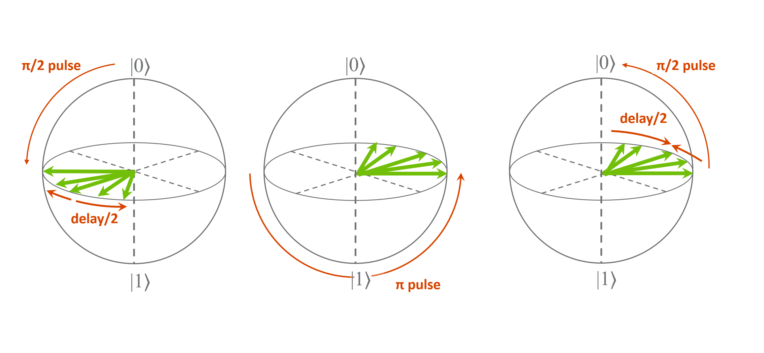
The experiment therefore follows the following steps:

1. Initialize the qubit to an equal superposition state between the ground and excited state (in the \(XY\) plane of the Bloch sphere) by applying a \(\frac{\pi}{2}\) gate.

2. Apply a delay.

3. Apply a \(Z\) rotation to offset the natural precession.

4. Apply a second \(\frac{\pi}{2}\) gate to drive the qubit toward either the ground or excited state.

5. Measure the population of the qubit in the excited state.

6. Repeat the above steps with varying delay time.

We start again by initializing a qubit and loading a channel mapper to create a new instance of the EchoExperiment class. Next, we generate a calibration set for the qubit using make_calibration_set(). This file includes the quantum operations and variables we will need to run the experiment.

# set the following to True when connected to hardware
run_on_hw = False

n_qubits = 1
qubits = qcs.Qudits(range(n_qubits))
calibration_set = make_calibration_set(n_qubits)

# generate an empty channel mapper
mapper = qcs.ChannelMapper("ip_addr")

# create Ramsey experiment
echo_experiment = EchoExperiment(mapper, calibration_set=calibration_set, qubits=qubits)

echo_experiment.draw()

# The program consists of two `X90` gates, with a `X` gate placed between them.
# There are two delays of `d/2` where `d` is variable, one in between the first
# `X90` gates and the `X` gate and one in between the `X` gates and the second
# `X90` gate. The sequence is then followed by a measurement.
#

		Program Program Duration undefined Layers 1 Targets 1 Repetitions
		Layer #0 Layer #0 Duration undefined
qudits	0	X90 Gate X90 on ('qudits', 0) Matrix: 0.71 -0.71j -0.71j 0.71	Delay on ('qudits', 0) Parameters Duration Array(name=pulse_delay, shape=(1,), dtype=float, unit=s)	X Gate X on ('qudits', 0) Matrix: 0 1 1 0	Delay on ('qudits', 0) Parameters Duration Array(name=pulse_delay, shape=(1,), dtype=float, unit=s)	X90 Gate X90 on ('qudits', 0) Matrix: 0.71 -0.71j -0.71j 0.71	Measure on ('qudits', 0) Parameters Dim 2

# configure the repetitions for this experiment
start_delay = 40e-9
end_delay = 80e-9
steps = 3
scan_values = np.linspace([start_delay] * n_qubits, [end_delay] * n_qubits, steps)
echo_experiment.configure_repetitions(delays=scan_values, n_shots=1)

Compiling this program to the waveform level using the ParameterizedLinkers in the calibration set results in the following program: echo_experiment.compiled_program.render(channel_subplots=False, sample_rate=5e9)

To execute this experiment, we can simply run

if run_on_hw:
    echo_experiment.execute()
else:
    # load in a previously executed version of this experiment
    echo_experiment = qcs.load("EchoExperiment_data.hdf5")

The draw and plot methods can then be used just like for the Ramsey experiment. echo_experiment.draw()

echo_experiment.plot_trace(channels=qcs.Qudits(1, "ancilla"))

---

Download

Download this file as Jupyter notebook: qubit_coherence.ipynb.

On this page