Download

Download this file as Jupyter notebook: dispersive_shift.ipynb.

Dispersive Shift

In the dispersive regime, the qubit-resonator detuning \(\Delta\) = \(\omega_q\) - \(\omega_r\) is much larger than the coupling strength g. In this regime the qubit and the resonator do not exchange energy directly, instead the resonator’s frequency changes depending on the qubit state. This is what allows the measurement of the qubit’s state without disturbing it. In this regime the Hamiltonian can be rewritten in the following form:

\[H = \hbar(\omega_r + \chi\sigma_z)a^{\dagger}a + \frac{1}{2}\hbar(\omega_q + \chi)\sigma_z\]

Where we introduced the dispersive shift:

\[\chi = \frac{g^2}{\Delta}\]

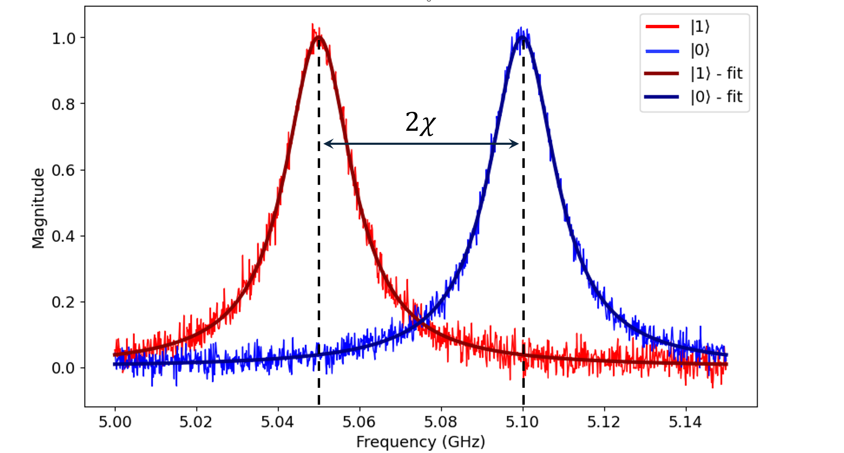
This parameter is what we are characterizing in this guide with the help of the the DispersiveShift class. To determine the dispersive shift, we are essentially performing two resonator spectroscopy experiments, with the qubit in either the ground or the excited state. The procedure is as follows:

Initialize the qudit to the ground state.

Either leave the qubit in the ground state or apply a control pulse to bring the qubit to the excited state.

Apply a readout pulse at a frequency \(\omega\) on the target qudit.

Repeat the above steps for different values of \(\omega\).

The result will be two lorentzian peaks separated by \(2\chi\) like so:

[2]:

# Import the necessary packages
import numpy as np
import keysight.qcs as qcs
from keysight.qcs.experiments import DispersiveShift, make_calibration_set

We start by initializing a qubit and loading a channel mapper, which links up to the hardware channels. If a channel mapper doesn’t exist, we can create a new one and add the hardware references to it. Next, we generate a calibration set for the qubit using make_calibration_set(). This file includes the quantum operations and variables we will need to run the experiment.

[3]:

# set the following to True when connected to hardware
run_on_hw = False

n_qubits = 1
qubits = qcs.Qudits(range(n_qubits))

# Set this to True if channel mapper exists
channel_mapper_exists = False

if channel_mapper_exists:
    mapper = qcs.load("<path/to/channel_mapper.qcs>")
else:
    # generate an empty channel mapper with the correct ip address
    mapper = qcs.ChannelMapper("<ip address>")

calibration_set = make_calibration_set(qubits=n_qubits)

We can now create a new instance of the DispersiveShift class. We use the draw() method to visualize the experiment program that will be executed on hardware.

[4]:

# Create a Dispersive Shift experiment
dispersive_experiment = DispersiveShift(
    mapper, calibration_set=calibration_set, qubits=qubits
)

dispersive_experiment.draw()

Program

Layer #0

qudits

0

RX

The program consists of the waveform representing our RX gate on the control channel that is mapped to the qubit. Note that in this representation, the virtual qubit and control channels appear separate, but after final compilation through the whole calibration set, they will be merged into the same channel.

To configure the repetitions of this experiment, we sweep the frequency of the RX waveform.

Note

Note that the name of the control frequencies stored in the calibration set is xy_pulse_frequencies.

[5]:

# Specify the frequency range for this experiment
start_frequency = 5.02e9
end_frequency = 5.05e9
steps = 10
scan_values = np.linspace(
    [start_frequency] * len(qubits), [end_frequency] * len(qubits), steps
)

# Specify the ``RX`` Gate amplitudes to be applied
x_amplitudes = qcs.Array(
    name="x_amplitudes", value=np.transpose([[0, np.pi]] * len(qubits))
)

# Configure the repetitions for the experiment
dispersive_experiment.configure_repetitions(
    x_amplitudes=x_amplitudes, frequencies=scan_values, n_shots=1
)

Compiling this program to the waveform level using the ParameterizedLinkers in the calibration set results in the following program:

[6]:

dispersive_experiment.draw()

Program

Layer #0

qudits

0

RX

We again use the render method to visualize this with the ChannelMapper.

[7]:

dispersive_experiment.compiled_program.render(
    channel_subplots=False,
    lo_frequency=5e9,
    sweep_index=(9, 1),
    sample_rate=5e9,
)

To execute this experiment, we can simply run

[8]:

if run_on_hw:
    dispersive_experiment.execute()
else:
    # load in a previously executed version of this experiment
    dispersive_experiment = qcs.load("DispersiveShift.qcs")

For the purposes of this demonstration, we added an “ancilla” qubit to the Dispersive Shift program and connected the physical output channels for our qubit to the digizer associated with the ancilla to allow us to capture the control pulse.

[9]:

dispersive_experiment.draw()

Program

Layer #0

qudits

0

RX

ancilla

1

The ancilla qubit is mapped to the digitizer channel 1 and has a single acquisition that spans the duration of the control pulse.

[10]:

dispersive_experiment.plot_trace()

Here we can see the frequencies of the control pulse being updated at each point in the sweep. Note that our local oscillator (LO) frequency was set to 5 GHz for this example.

Download

Download this file as Jupyter notebook: dispersive_shift.ipynb.

On this page