Qubit Spectroscopy#
Quantum computers store information in the discrete energy levels of qudits. To process this information, they perform operations that alter the energetic state of these qudits. For example, by exciting the electromagnetic field in the vicinity of a qudit at the frequency corresponding to the difference between the energy levels, quantum computers can drive a transition between two energy levels of the qudit and perform operations such as Pauli-X gates.
When assembling a quantum computer, it is important to learn the energy gap between different levels of the available qudits to be able to perform accurate quantum operations. This is typically done by running a spectroscopy experiment.
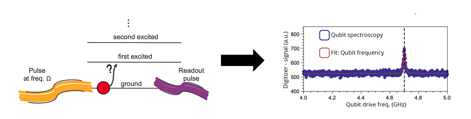
In order to learn the energy gap between the ground state and the first excited state of a qudit, a spectroscopy experiment undertakes the following steps:
Initialize the qudit to the ground state.
Apply a control pulse at a frequency \(\omega\) on the target qudit.
Measure the population of the qudit in the excited state.
Repeat the above steps for different values of \(\omega\).
Select the frequency which maximizes the population in the excited state.
The population of the excited state gives a resonance curve, where the energy gap can be deduced from the frequency with the highest population in the excited state.
Note
The above steps can be applied directly to any two levels of a qudit, for example to learn the energy gap between the first and the second excited states in the figure above.
[2]:
import keysight.qcs as qcs
import numpy as np
We start by initializing a qubit and defining an empty channel mapper to create a new
instance of the QubitSpectroscopy class. We load
a pre-defined CalibrationSet that contains a
configuration for up to 10 qubits and linkers for the RX and measurement
gates.
Because the purpose of this experiment is to calibrate a parameter, namely the control
frequency of the qubit, the QubitSpectroscopy is
a subclass of the more generic
CalibrationExperiment which requires an
operation name to be passed on instantiation. This name must match the name with which
the associated ParameterizedLinker is stored in
the calibration set.
[3]:
from keysight.qcs.experiments import QubitSpectroscopy, make_calibration_set
from simulated_experiments.simulated_experiments import SimulatedSpectroscopyExperiment

# set the following to True when connected to hardware
run_on_hw = False

n_qubits = 1
calibration_set = make_calibration_set(n_qubits)
qubits = qcs.Qudits(range(n_qubits))

# generate an empty channel mapper
mapper = qcs.ChannelMapper("127.0.0.1")

# the operation that we are calibrating here is for the RX gate
operation = "x"

# create spectroscopy experiment
spectroscopy_exp = QubitSpectroscopy(
    mapper,
    calibration_set=calibration_set,
    qubits=qubits,
    operation=operation,
)

spectroscopy_exp.draw()
|
Program
|
||||||||||||||||||||||||||||||||||||||
|
||||||||||||||||||||||||||||||||||||||
The program consists of the waveform representing our RX gate on the control
channel that is mapped to the qubit. Note that in this representation, the virtual
qubit and control channels appear separate, but after final compilation
through the whole calibration set, they will be merged into the same channel.
To configure the repetitions of this experiment, we sweep the frequency of the RX
waveform. Note that the name of the control frequencies stored
in the calibration set is xy_pulse_frequencies.
[4]:
# configure the repetitions for this experiment
current_freq = spectroscopy_exp.calibration_set.variables.xy_pulse_frequencies[0].value

start_frequency = current_freq - 200e6
end_frequency = current_freq + 200e6
steps = 9
scan_values = np.linspace(start_frequency, end_frequency, steps)


spectroscopy_exp.configure_repetitions(
    frequencies=scan_values, n_shots=1, frequency_name="xy_pulse_frequencies"
)
Compiling this program to the waveform level using the
ParameterizedLinkers in the calibration set
results in the following program:
[5]:
spectroscopy_exp.draw()
|
Program
|
||||||||||||||||||||||||||||||||||||||||||||||||
|
||||||||||||||||||||||||||||||||||||||||||||||||
We again use the render method to visualize this with the
ChannelMapper.
[6]:
spectroscopy_exp.compiled_program.render(
    channel_subplots=False,
    lo_frequency=5e9,
    sweep_index=5,
    sample_rate=5e9,
)
To execute this experiment, we can simply run
[7]:
if run_on_hw:
    spectroscopy_exp.execute()
else:
    # load in a previously executed version of this experiment
    spectroscopy_exp = qcs.load("QubitSpectroscopy.qcs")
For the purposes of this demonstration, we added a second “ancilla” qubit to the Ramsey program and connected the physical output channels for our qubit to the digitizer associated with the ancilla to allow us to capture the control pulse.
[8]:
spectroscopy_exp.draw()
|
QubitSpectroscopy
|
||||||||||||||||||||||||||||||||||||||||||||||||||||||
|
||||||||||||||||||||||||||||||||||||||||||||||||||||||
The ancilla qubit is mapped to the digitizer channel 1 and has a single
acquisition that spans the duration of the control pulse.
[9]:
spectroscopy_exp.plot_trace(channels=qcs.Qudits(1, "ancilla"))
Here we can see the frequencies of the control pulse being updated at each point in the sweep. Note that our local oscillator (LO) frequency was set to 5 GHz for this example.
Fitting and calibration workflow#
Let’s walk through how to extract the qubit resonance frequency from the Qubit Spectroscopy experiment and how to update the corresponding variables in our calibration set. For this example, we load in an experiment with simulated data that was imported at the beginning of the file:
[10]:
spectroscopy_exp = SimulatedSpectroscopyExperiment(calibration_set, qubits)
[11]:
spectroscopy_exp.plot_iq(plot_type="linear")
[12]:
spectroscopy_exp.get_iq_array()
[12]:
<xarray.DataArray (qudit: 1, xy_pulse_frequencies: 100, shot: 1)> Size: 2kB
array([[[-0.02697363+0.02697231j],
        [-0.02698258+0.02697168j],
        [-0.0270156 +0.02697101j],
        [-0.02699067+0.02697032j],
        [-0.02700946+0.0269696j ],
        [-0.02697873+0.02696883j],
        [-0.02697701+0.02696803j],
        [-0.02699427+0.02696719j],
        [-0.02699698+0.0269663j ],
        [-0.02701681+0.02696536j],
        [-0.02701268+0.02696437j],
        [-0.02699923+0.02696331j],
        [-0.02700648+0.0269622j ],
        [-0.02699832+0.02696102j],
        [-0.02700226+0.02695976j],
        [-0.02698675+0.02695841j],
        [-0.02699197+0.02695698j],
        [-0.02700278+0.02695544j],
        [-0.02698196+0.02695379j],
        [-0.02702298+0.02695202j],
...
        [-0.02698938+0.02703474j],
        [-0.02699587+0.02703379j],
        [-0.02696801+0.0270329j ],
        [-0.02698231+0.02703205j],
        [-0.0269789 +0.02703125j],
        [-0.02697568+0.02703048j],
        [-0.02700757+0.02702975j],
        [-0.02701645+0.02702905j],
        [-0.02698409+0.02702839j],
        [-0.02698149+0.02702775j],
        [-0.02699121+0.02702715j],
        [-0.02699119+0.02702657j],
        [-0.02702966+0.02702601j],
        [-0.02700405+0.02702548j],
        [-0.02697612+0.02702496j],
        [-0.02702001+0.02702447j],
        [-0.02698118+0.027024j  ],
        [-0.02696806+0.02702354j],
        [-0.02700288+0.0270231j ],
        [-0.02699568+0.02702268j]]])
Coordinates:
  * qudit                 (qudit) <U38 152B 'Qudits(labels=[0], name=qudits, ...
  * xy_pulse_frequencies  (xy_pulse_frequencies) float64 800B 4.9e+09 ... 5.3...
* shot (shot) int64 8B 0The fit() method takes this I/Q data
and fits it to a complex lorentzian model, as specified by the built-in
ComplexLorentzian.
The result of the fit is an EstimateCollection,
which contains individual Estimates for each
qubit that was fitted.
[13]:
ec = spectroscopy_exp.fit()
print(ec)
print(ec.estimates[0])
EstimateCollection(1)
Estimate(amplitude=0.0004928379821974705, resonance=5079874827.71701, kappa=20192703.44965815, offset_real=-0.026998524628909344, ...)
The fitted and the pre-processed data can be visualized by calling the
plot() method:
[14]:
spectroscopy_exp.plot()
We can then get the calibration value associated to this Spectroscopy Experiment by
calling
get_updated_calibration_values().
This method will compute the new values for the calibration variable(s) of this
experiment using the fit results.
[15]:
spectroscopy_exp.get_updated_calibration_values()
[15]:
{'xy_pulse_frequencies': [5079874827.71701]}
To check the current state of that variable in the calibration_set to confirm its update, one can do:
[16]:
spectroscopy_exp.calibration_set.variables.xy_pulse_frequencies.value
[16]:
array([5.1e+09])
The update is then done as follows:
[17]:
spectroscopy_exp.set_updated_calibration_values()
spectroscopy_exp.calibration_set.variables.xy_pulse_frequencies.value
[17]:
array([5.07987483e+09])
The last line printing the new updated value, thus confirming that the update has been successful.