---

Download

Download this file as Jupyter notebook: qubit_rabi.ipynb.

Rabi experiment

This guide shows how to perform a Rabi experiment to calibrate a \(\pi\)-pulse using a program. This experiment can be easily generated using the RabiExperimentclass.

The Rabi experiment is the second step in calibrating our first quantum gates. Following the Qubit spectroscopy experiment, we learned the energy gap between the ground state and first excited state of our two-level system. In other words, we have determined the resonance frequency of our qubit, and can now apply pulses at this frequency to alter the qubit’s state.

The state of the qubit can be visualized using the Bloch sphere. The ground state \(|0\rangle\) is represented by the north pole, and the excited state \(|1\rangle\) is represented by the south pole as shown. By applying pulses of varying strengths to a qubit in the ground state, we can drive a rotation around the Bloch sphere by some as-yet-unknown angles.

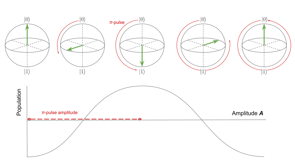
A rotation of \(\pi\) takes us from \(|0\rangle\) to \(|1\rangle\), which is the operation implemented by a Pauli-X gate. The pulse that drives this rotation is called a \(\pi\)-pulse. Here we assume that the pulse duration is fixed, and we will vary strength by varying pulse amplitude. Our goal is to learn the required \(\pi\)-pulse amplitude, in order to calibrate our gate.

To learn the pulse amplitude, we perform a Rabi experiment as follows:

1. Initialize the qubit to the ground state.

2. Apply a control pulse with the resonance frequency \(\omega_r\) and amplitude \(A\), for a fixed duration, on the target qubit.

3. Measure the population of the qubit in the excited state.

4. Repeat the above steps with varying amplitude \(A\).

The observed population as a function of amplitude will be a sinusoid, corresponding to rotations around the Bloch sphere. We can read off the \(\pi\)-pulse amplitude as half the period of the observed oscillation.

import keysight.qcs as qcs
import numpy as np

We start by initializing a qubit and defining an empty channel mapper to create a new instance of the RabiExperiment class. We load a make_calibration_set function that creates a calibration set for the given amount of qubit containing the linkers for the RX , Z and measurement gates. Lastly, we import an experiment with simulated data to demonstrate the fitting and calibration workflow at the end of this file.

from keysight.qcs.experiments import RabiExperiment, make_calibration_set
from simulated_experiments.simulated_experiments import SimulatedRabiExperiment

# set the following to True when connected to hardware
run_on_hw = False

n_qubits = 1
calibration_set = make_calibration_set(n_qubits)
qubits = qcs.Qudits(range(n_qubits))

# generate an empty channel mapper
mapper = qcs.ChannelMapper("ip_addr")

# create Rabi experiment
rabi_experiment = RabiExperiment(mapper, calibration_set=calibration_set, qubits=qubits)

rabi_experiment.program.draw()

# The program consists of a simple `RX` gate with variable amplitude followed by a
# measurement. During execution, we set the amplitude of this gate to a range of values
# from zero to one.

		Program Program Duration undefined Layers 2 Targets 2 Repetitions
		Layer #0 Layer #0 Duration 30 ns	Layer #1 Layer #1 Duration undefined
xy_pulse	0	RFWaveform on ('xy_pulse', 0) Parameters Duration ScalarRef(name=xy_pulse_durations, value=30 ns, dtype=float, unit=s) Amplitude ScalarRef(name=x180_pulse_amplitudes, value=0.5, dtype=float, unit=none) Frequency ScalarRef(name=xy_pulse_frequencies, value=5.1 GHz, dtype=float, unit=Hz) Envelope GaussianEnvelope(2.0) Instantaneous Phase ScalarRef(name=x_phase, value=0 rad, dtype=float, unit=rad) Post-phase ScalarRef(name=x_post_phase, value=0 rad, dtype=float, unit=rad)
qudits	0		Measure on ('qudits', 0) Parameters Dim 2

# configure the repetitions for this experiment
start_amplitude = 0
end_amplitude = 1
steps = 10
scan_values = np.linspace(start_amplitude, end_amplitude, steps)
rabi_experiment.configure_repetitions(amplitudes=scan_values, n_shots=1)

Compiling this program to the waveform level using the ParameterizedLinkers in the calibration set results in the following program:

rabi_experiment.compiled_program.draw()

		Program Program Duration 130 ns Layers 2 Targets 3 Repetitions Repeat with 1 repetitions Sweep with 10 repetitions Associations x180_pulse_amplitudes Array(name=_implicit, shape=(10,), dtype=float, unit=none, value=[0, 0.1111, 0.2222, 0.3333, 0.4444, 0.5556, 0.6667, 0.7778, 0.8889, 1])
		Layer #0 Layer #0 Duration 30 ns	Layer #1 Layer #1 Duration 100 ns
xy_pulse	0	RFWaveform on ('xy_pulse', 0) Parameters Duration ScalarRef(name=xy_pulse_durations, value=30 ns, dtype=float, unit=s) Amplitude ScalarRef(name=x180_pulse_amplitudes, value=0.5, dtype=float, unit=none) Frequency ScalarRef(name=xy_pulse_frequencies, value=5.1 GHz, dtype=float, unit=Hz) Envelope GaussianEnvelope(2.0) Instantaneous Phase ScalarRef(name=x_phase, value=0 rad, dtype=float, unit=rad) Post-phase ScalarRef(name=x_post_phase, value=0 rad, dtype=float, unit=rad)
readout_pulse	0		RFWaveform on ('readout_pulse', 0) Parameters Duration ScalarRef(name=readout_pulse_duration, value=100 ns, dtype=float, unit=s) Amplitude ScalarRef(name=readout_pulse_amplitudes, value=0.1, dtype=float, unit=none) Frequency ScalarRef(name=readout_frequencies, value=5.15 GHz, dtype=float, unit=Hz) Envelope SineEnvelope() Instantaneous Phase ScalarRef(name=measurement_phase, value=0 rad, dtype=float, unit=rad) Post-phase ScalarRef(name=measurement_post_phase, value=0 rad, dtype=float, unit=rad)	Delay on ('readout_pulse', 0) Parameters Duration Scalar(name=_implicit, value=0 s, dtype=float, unit=s)
readout_acquisition	0		Acquisition on ('readout_acquisition', 0) Parameters Duration ScalarRef(name=acquisition_duration, value=100 ns, dtype=float, unit=s) Integration Filter RFWaveform Parameters Duration ScalarRef(name=acquisition_duration, value=100 ns, dtype=float, unit=s) Amplitude ScalarRef(name=measurement_integrator_amplitude, value=1, dtype=float, unit=none) Frequency ScalarRef(name=readout_frequencies, value=5.15 GHz, dtype=float, unit=Hz) Envelope ConstantEnvelope() Instantaneous Phase ScalarRef(name=measurement_integrator_phase, value=0 rad, dtype=float, unit=rad) Post-phase ScalarRef(name=measurement_integrator_post_phase, value=0 rad, dtype=float, unit=rad) Classifier Classifier(Array(name=references, shape=(1, 2), dtype=complex, unit=none))	Delay on ('readout_acquisition', 0) Parameters Duration Scalar(name=_implicit, value=0 s, dtype=float, unit=s)

We again use the render method to visualize this with the ChannelMapper.

rabi_experiment.compiled_program.render(
    channel_subplots=False,
    lo_frequency=5e9,
    sweep_index=5,
    sample_rate=5e9,
)

To execute this experiment, we can simply run

if run_on_hw:
    rabi_experiment.execute()
else:
    # load in a previously executed version of this experiment
    rabi_experiment = qcs.load("RabiExperiment.qcs")

For the purposes of this demonstration, we added a second “ancilla” qubit to the Rabi program and connected the physical output channels for our qubit control to the digizer associated with the ancilla to allow us to capture both the control and the readout pulse.

rabi_experiment.draw()

		Program Program Duration undefined Layers 2 Targets 3 Repetitions Sweep with 10 repetitions Associations x180_pulse_amplitudes Array(name=_implicit, shape=(10,), dtype=float, unit=none, value=[0, 0.1111, 0.2222, 0.3333, 0.4444, 0.5556, 0.6667, 0.7778, 0.8889, 1]) Repeat with 1 repetitions
		Layer #0 Layer #0 Duration undefined	Layer #1 Layer #1 Duration undefined
xy_pulse	0	RFWaveform on ('xy_pulse', 0) Parameters Duration ScalarRef(name=xy_pulse_durations, value=30 ns, dtype=float, unit=s) Amplitude ScalarRef(name=x180_pulse_amplitudes, value=0.5, dtype=float, unit=none) Frequency ScalarRef(name=xy_pulse_frequencies, value=5.1 GHz, dtype=float, unit=Hz) Envelope GaussianEnvelope(2.0) Instantaneous Phase ScalarRef(name=x_phase, value=0 rad, dtype=float, unit=rad) Post-phase ScalarRef(name=x_post_phase, value=0 rad, dtype=float, unit=rad)
ancilla	1	Measure on ('ancilla', 1) Parameters Dim 2
qudits	0		Measure on ('qudits', 0) Parameters Dim 2

rabi_experiment.compiled_program.draw()

		Program Program Duration 145 ns Layers 2 Targets 4 Repetitions Sweep with 10 repetitions Associations x180_pulse_amplitudes Array(name=_implicit, shape=(10,), dtype=float, unit=none, value=[0, 0.1111, 0.2222, 0.3333, 0.4444, 0.5556, 0.6667, 0.7778, 0.8889, 1]) Repeat with 1 repetitions
		Layer #0 Layer #0 Duration 45 ns	Layer #1 Layer #1 Duration 100 ns
xy_pulse	0	RFWaveform on ('xy_pulse', 0) Parameters Duration ScalarRef(name=xy_pulse_durations, value=30 ns, dtype=float, unit=s) Amplitude ScalarRef(name=x180_pulse_amplitudes, value=0.5, dtype=float, unit=none) Frequency ScalarRef(name=xy_pulse_frequencies, value=5.1 GHz, dtype=float, unit=Hz) Envelope GaussianEnvelope(2.0) Instantaneous Phase ScalarRef(name=x_phase, value=0 rad, dtype=float, unit=rad) Post-phase ScalarRef(name=x_post_phase, value=0 rad, dtype=float, unit=rad)
readout_acquisition	0		Acquisition on ('readout_acquisition', 0) Parameters Duration ScalarRef(name=acquisition_duration, value=100 ns, dtype=float, unit=s) Integration Filter RFWaveform Parameters Duration ScalarRef(name=acquisition_duration, value=100 ns, dtype=float, unit=s) Amplitude ScalarRef(name=measurement_integrator_amplitude, value=1, dtype=float, unit=none) Frequency ScalarRef(name=readout_frequencies, value=5.15 GHz, dtype=float, unit=Hz) Envelope ConstantEnvelope() Instantaneous Phase ScalarRef(name=measurement_integrator_phase, value=0 rad, dtype=float, unit=rad) Post-phase ScalarRef(name=measurement_integrator_post_phase, value=0 rad, dtype=float, unit=rad) Classifier Classifier(Array(name=references, shape=(1, 2), dtype=complex, unit=none))	Delay on ('readout_acquisition', 0) Parameters Duration Scalar(name=_implicit, value=0 s, dtype=float, unit=s)
	1	Acquisition on ('readout_acquisition', 1) Parameters Duration Scalar(name=_implicit, value=45 ns, dtype=float, unit=s) Integration Filter DCWaveform Parameters Duration Scalar(name=_implicit, value=45 ns, dtype=float, unit=s) Amplitude 1 Frequency 0 Hz Envelope ConstantEnvelope() Instantaneous Phase 0 Post-phase 0
readout_pulse	0		RFWaveform on ('readout_pulse', 0) Parameters Duration ScalarRef(name=readout_pulse_duration, value=100 ns, dtype=float, unit=s) Amplitude ScalarRef(name=readout_pulse_amplitudes, value=0.1, dtype=float, unit=none) Frequency ScalarRef(name=readout_frequencies, value=5.15 GHz, dtype=float, unit=Hz) Envelope SineEnvelope() Instantaneous Phase ScalarRef(name=measurement_phase, value=0 rad, dtype=float, unit=rad) Post-phase ScalarRef(name=measurement_post_phase, value=0 rad, dtype=float, unit=rad)	Delay on ('readout_pulse', 0) Parameters Duration Scalar(name=_implicit, value=0 s, dtype=float, unit=s)

The ancilla qubit is mapped to the digitizer channel 1 and has a single acquisition that spans the duration of the control pulse.

rabi_experiment.plot_trace()

Here we can see the control pulse with our varying amplitudes. Note that our local oscillator (LO) frequency was set to 5 GHz for this example.

Fitting and calibration workflow

Let’s walk through how to extract the desired drive amplitude from the Rabi experiment and how to update the corresponding variables in our calibration set. For this example, we load in an experiment with simulated data that we imported at the beginning of the file:

rabi_experiment = SimulatedRabiExperiment(calibration_set, qubits)

rabi_experiment.plot_iq(plot_type="linear")

The fit() method takes this I/Q data and fits it to a decaying sinusoidal model, as specified by the built-in DecayingSinusoid. In order to specify how to prepare the I/Q data for fitting (in this case, we want to fit the magnitude), the RabiExperiment uses the IQuadrature pre-processor, which extracts the I quandrature out of the complex I/Q data.

The result of the fit is an EstimateCollection, which contains individual Estimates for each qubit that was fitted.

ec = rabi_experiment.fit()
print(ec)
print(ec.estimates[0])

EstimateCollection(1)
Estimate(amplitude=1.3380733832098393, decay_rate=2.1250154974935, frequency=39.84246404001343, phase=-1.5244173091736075, ...)

We can represent estimate parameters and its values and estimate collection in a tabular form by calling the draw() method:

ec.draw()

		Estimate Collection
		0
amplitude		1.33807 Estimate: amplitude val = 1.3380733832098393 std = 0.05624952904855688
decay_rate		2.12502 Estimate: decay_rate val = 2.1250154974935 std = 0.13913181097775268
frequency		39.84246 Estimate: frequency val = 39.84246404001343 std = 0.1364048600840517
offset		1.22284 Estimate: offset val = 1.2228380961930574 std = 0.012794041182882718
phase		-1.52442 Estimate: phase val = -1.5244173091736075 std = 0.039987548065996324

The fitted and the pre-processed data can be visualized by calling the plot() method:

rabi_experiment.plot()

We can then get the calibration value associated to this Rabi Experiment by calling get_updated_calibration_values(). This method will compute the new values for the calibration variable(s) of this experiment using the fit results.

rabi_experiment.get_updated_calibration_values()

{'x180_pulse_amplitudes': 0.05019769856581706}

To check the current state of that variable in the calibration_set to confirm its update, one can do:

rabi_experiment.calibration_set.variables.x180_pulse_amplitudes.value

array([0.5])

The update is then done as follows:

rabi_experiment.set_updated_calibration_values()
rabi_experiment.calibration_set.variables.x180_pulse_amplitudes.value

array([0.0501977])

The last line printing the new updated value, thus confirming that the update has been successful.

---

Download

Download this file as Jupyter notebook: qubit_rabi.ipynb.

On this page